Cells don’t function independently. They belong to a complex and interconnected network. This makes gene expression profiling of individual cells not enough for understanding their activities and crosstalk in the tissue context.
Like a marriage between imaging and RNA sequencing, Spatial Transcriptomics is a revolutionized method to map gene activity on specific locations of the tissue, using spatially barcoded, complementary DNA primers to capture RNA transcripts on each position of the tissue. Earlier this year, 10X Genomics introduced its Visium Spatial Transcriptomics system, a high-throughput spatial transcriptomics solution that incorporates ~5,000 spots of 55-µm in diameter containing arrayed oligonucleotide barcodes for capturing mRNA in tissue sections (Michaela Asp, 2020). Each spot can capture 1-10 cells, letting researchers see how cells are organized in relation to one another and their corresponding gene activities.
To help biologists easily visualize and analyze 10X Visium Spatial Transcriptomics data, we adopted the new Spatial Transcriptomics dashboard into BioTuring Browser (BBrowser). The dashboard helps scientists to interactively:
- Re-visualize derived layers/classification of glass slide spots with tSNE/UMAP
- Overlay gene expression of one or multiple genes on the spatial coordinates
- Compare gene expression among different layers
- Find layer-enriched expression signatures and biological processes/ pathways
- Find differentially expressed genes between any 2 layers or locations
The new Visium Spatial Transcriptomics module also opens a new branch of BioTuring Browser, allowing instant access to spatial transcriptomics datasets from publications in an interactive approach.
BBrowser is available for download at www.bioturing.com/bbrowser.
Below we re-analyze a sample 10X Visium spatial transcriptomics dataset from the mouse brain dataset in BBrowser to help you see the dashboard more clearly.
1. Input your data
BBrowser supports importing the spatial expression matrices as MTX. You need to provide a folder with exactly 3 files for gene expression information and 1 spatial folder:
- genes.tsv.gz (or features.tsv.gz)
- barcodes.tsv.gz
- matrix.mtx.gz
- a folder named “spatial”, containing the following files: aligned_fiducials.jpg, detected_tissue_image.jpg, tissue_hires_image.png, tissue_lowres_image.png, scalefactors_json.json and tissue_positions_list.csv
2. Visualize derived layers with tSNE
BBrowser supports viewing both t-SNE/UMAP and spatial images of the dataset at a time in multiple interactive windows. Selection of spots on a window can be reflected on another in real time.
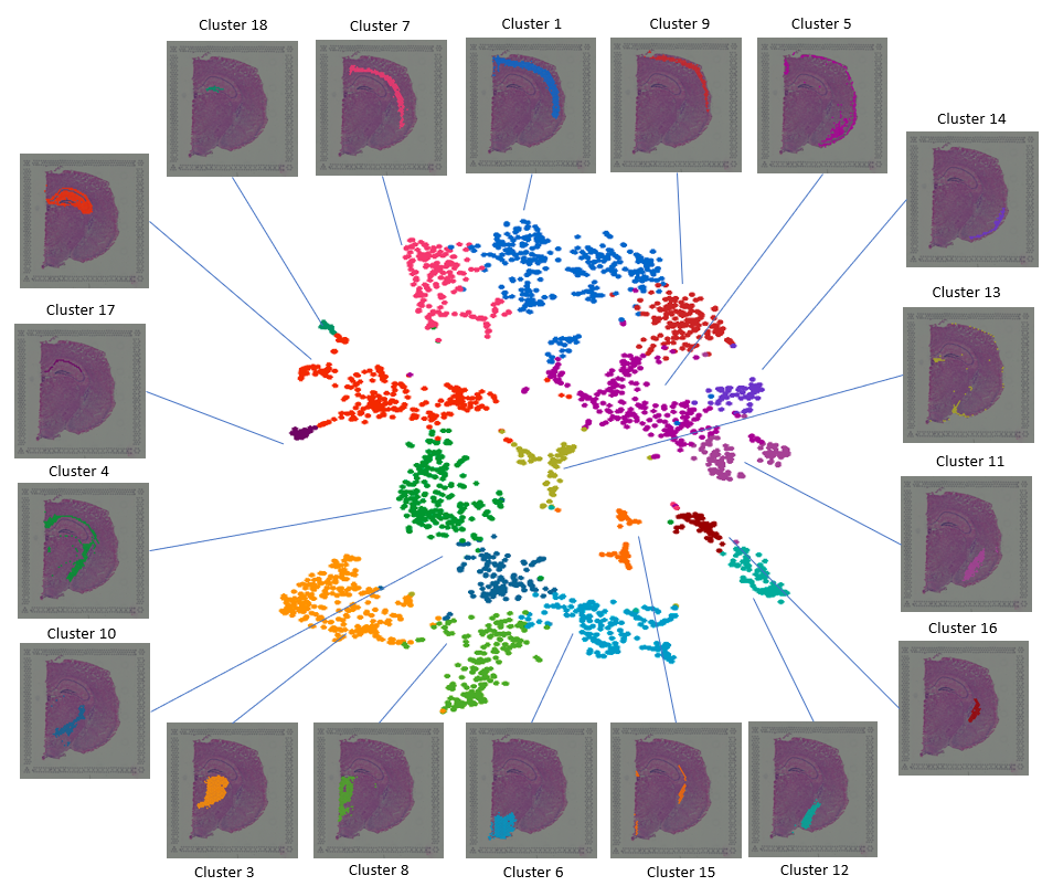
Figure 1. Visualizing layers of the mouse brain with the t-SNE plot and spatial images
3. Overlay one or multiple genes’ expression on the spatial coordinates
You can also see how a gene or multiple genes are expressed and correlated together on the spatial coordinates. Just type the gene name or its Ensembl ID or alias into the gene query box at the top and Enter.
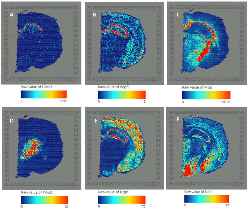
Figure 2. Query gene expression on the spatial image (A) Fibcd1; (B)Wipf3; (C) Mbp; (D) Prkcd; (E) Nrgn; (F) Ndn
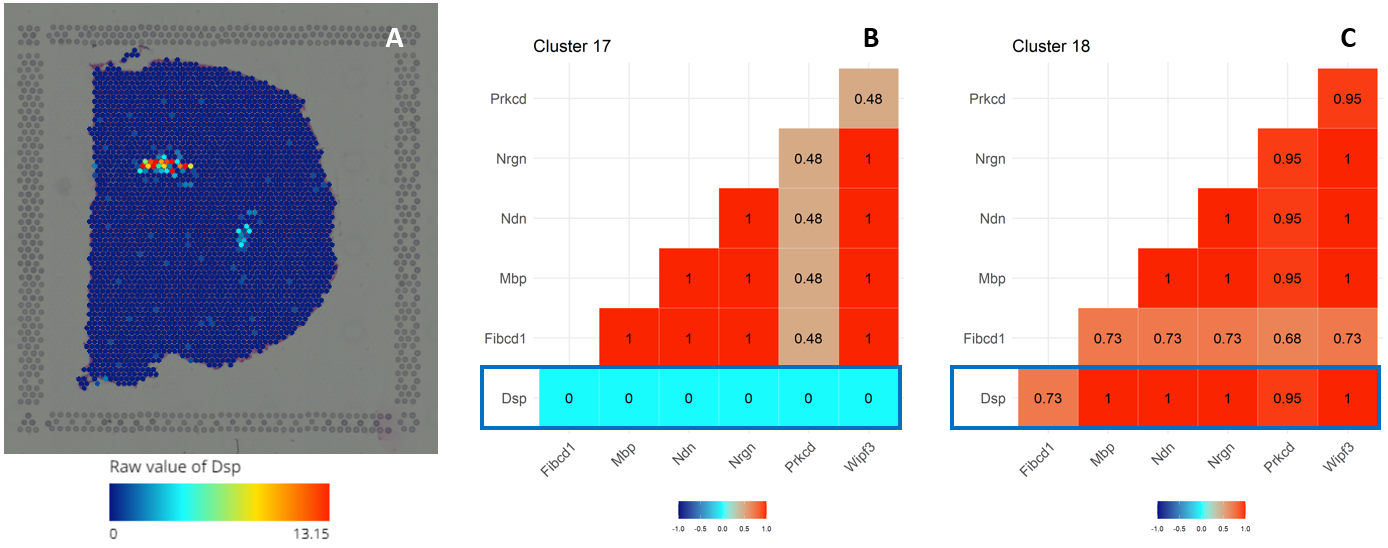
Figure 3. (A) Gene expression of Dsp. Correlations of Dsp expression with other genes (Fibcd1, Wipf3; ,Mbp, Prkcd, Nrgn, and Ndn) in (B) cluster 17 and (C) cluster 18
4. Compare gene expression among layers
Violin plots, box plots, bar plots, and heatmaps are available for easier comparison of gene expression among layers. The options can be found below the color bar when you query genes.
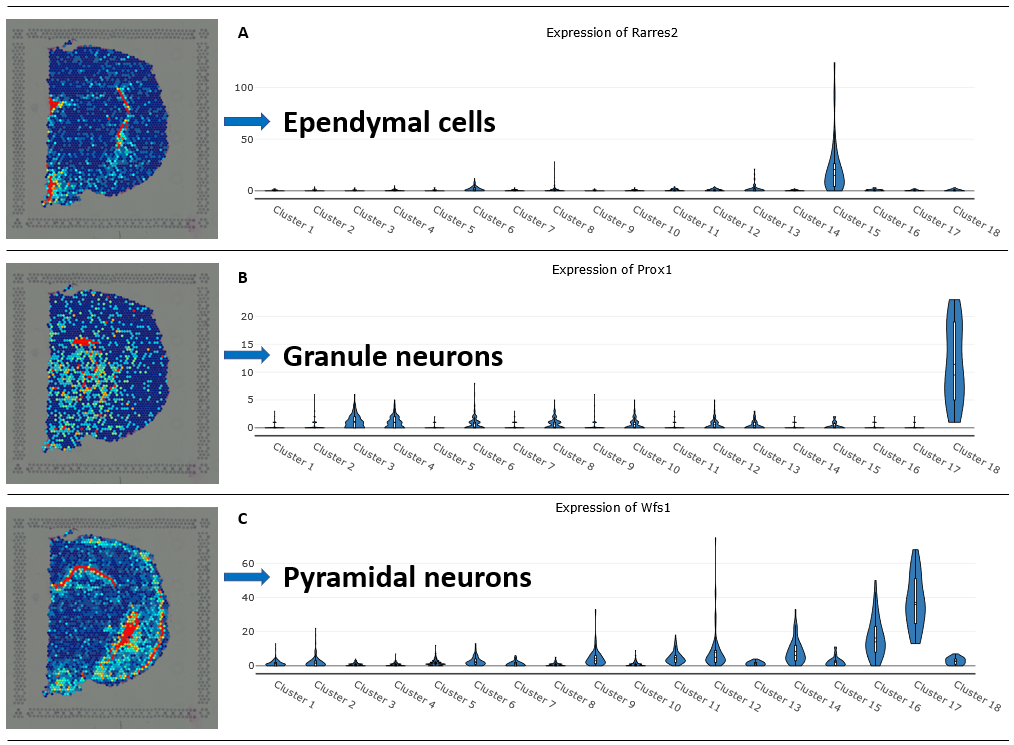
Figure 4. Studying gene expression patterns among clusters. (A) Rarres2 is a marker gene of ependymal cells and reaches the highest expression in Cluster 15. (B) Prox1 marks granule neurons, highest in Cluster 18, and (C) Wfs1 marks pyramidal neurons, highly expressed in cluster 12, 16, and 17 (Alma Andersson 2020)
5. Find extensive layer-enriched expression signatures and processes
To find a list of marker genes for all layers or clusters, simply hit the Find markers button. BBrowser also supports you to create a heatmap for all the top marker genes. You can also study enriched processes in a layer using the Enrichment Analysis option.
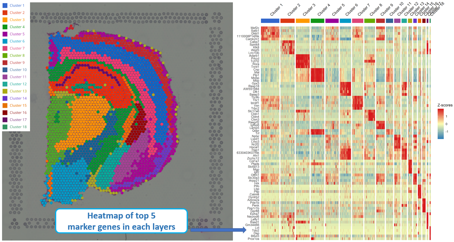
Figure 5. Heatmap of top 5 marker genes in each layer
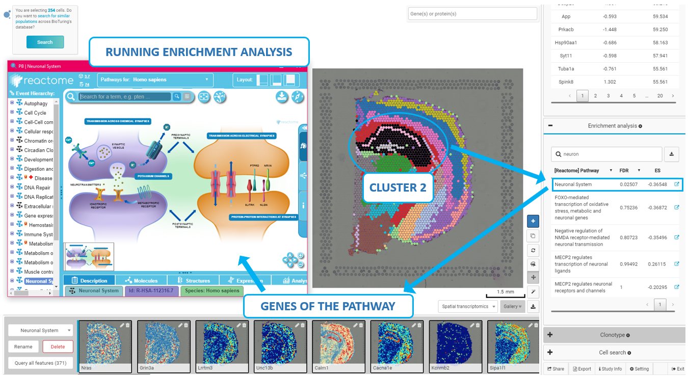
Figure 6. Finding enriched processes in a layer
6. Find differentially expressed genes between 2 layers
The differential expression analysis lets you compare any two layers and find the differentially expressed genes. The example shows the differentially expressed genes between cluster 1 and cluster 2, including Mef2c, Stmn1, Arpp19, Snap25…
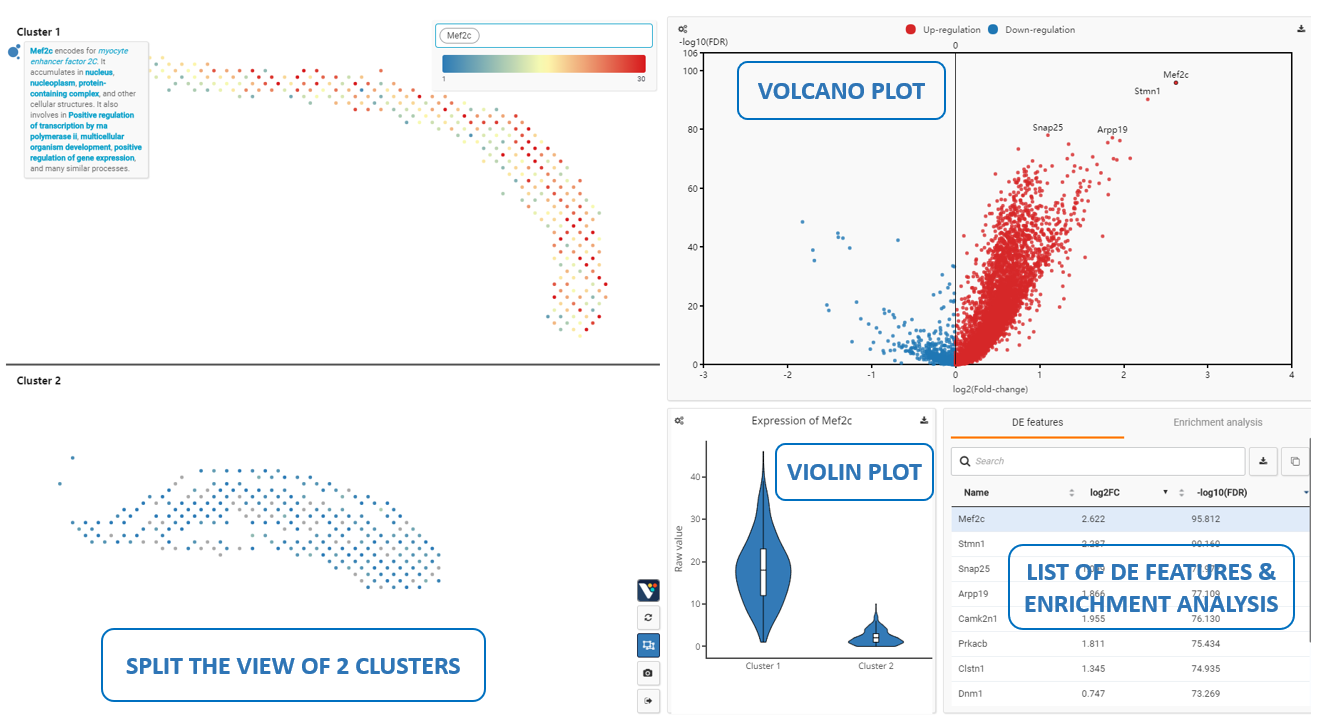
Figure 7. Running differential expression analysis on any two layers/cluster (e.g.Cluster 1 and Cluster 2)
BBrowser is now available for download at www.bioturing.com/bbrowser . The platform also supports single-cell RNA-seq data and CITE-seq data analysis.
Documentation: https://bioturing.com/document#spatial-transcriptomics
Tutorial video: https://youtu.be/0xzyv-nlcwE
References
1.Michaela Asp, Joseph Bergenstråhle, Joakim Lundeberg. (2020). Spatially Resolved Transcriptomes—Next Generation Tools for Tissue Exploration. BioEssays, Volume 42, Issue 10, https://doi.org/10.1002/bies.201900221.
2.Alma Andersson, Joseph Bergenstråhle, Michaela Asp, Ludvig Bergenstråhle, Aleksandra Jurek, José Fernández Navarro & Joakim Lundeberg. (2020). Single-cell and spatial transcriptomics enables probabilistic inference of cell type topography. Communications Biology, 3:565, https://doi.org/10.1038/s42003-020-0124.