Cellular state often exists in a continuum rather than distinct phases. A prime example is cell development and differentiation. With single-cell RNA-Seq, researchers can observe this continuum of transcriptomic changes via analysis of individual cells. The need to computationally model these dynamics leads to the birth of single-cell RNA-seq trajectory analysis methods (also known as “trajectory inference” or “pseudotime analysis”).

In this article, we’ll give you a broad review of Single-cell Trajectory analysis, important considerations, and a brief guideline on picking a suitable method.

Single-cell RNA-Seq Trajectory Analysis in a nutshell

A common question in biology is how cells differentiate from one state into various different states. This question not only matters in developmental biology, but it’s also vital in learning how cells transform during biological processes, such as the formation of tumor, aging, immune responses, etc.

Single-cell RNA-seq prompted a way to answer such questions. By analyzing and comparing the transcriptomic profiles of individual cells, we can, theoretically, reconstruct a “trajectory” – a path – that describes how cells traverse through different states. Cells are placed on this path based on the value of “pseudotime” – a number representing a cell’s relative position on the trajectory (it has nothing to do with real time points). The principle of reconstruction is: increasing “pseudotime” placing cells further away from the root.

The trajectory can be as simple as a path connecting one cell type to another, or as complex as a tree with multiple branches. The general workflow of a single-cell trajectory analysis is summarized in Figure 1. There are multiple tools to perform single-cell trajectory analysis. They generally follow the same workflow and mainly differ in trajectory reconstruction. In particular, the difference is in how tools analyze changes in cells’ transcriptomes as a function of pseudotime and map that information into a trajectory.

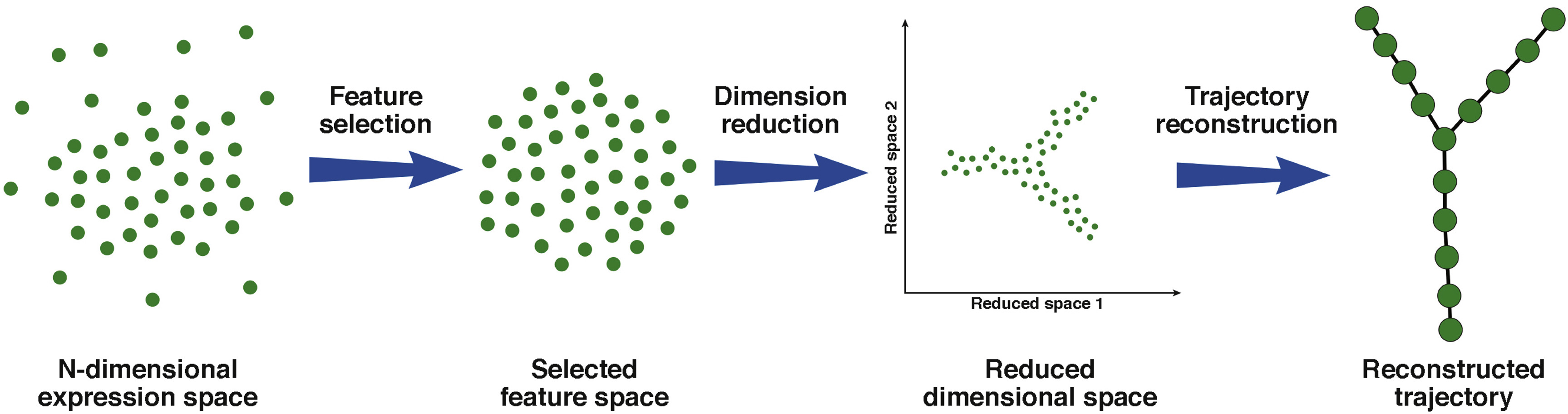
Figure 1. General workflow of most single-cell RNA-Seq trajectory analysis tools. Raw data in the high dimensional space will undergo feature selection and dimensionality reduction, revealing possible trajectory. Individual cells are then mapped onto this trajectory (Herring et al., 2018)

The Most Important Thing about Single-cell RNA-Seq Trajectory Analysis: Make sure your trajectory exists!

Before running, you should know or have substantial evidence that a trajectory exists. Some clues include the existence of intermediate states or transitional cell types in your data, the presence of a continuum of states among cells. During the trajectory analysis workflow, after dimensionality reduction, t-SNE/ UMAP plots can be somewhat useful to decide whether or not a trajectory analysis should follow.

Most often, the nature of your dataset and the biological foundation will be the strongest clue. If you are examining a dataset of stem cells differentiation, a trajectory analysis is a logical thing to do. However, if your data exists as distinct clusters and the cell types are not related by any known biological process, trajectory analysis may not be accurate.

Below are 2 examples demonstrating the importance of this point.

Example #1 (Figure 2): Figure 2 (upper) is the UMAP plot for Pellin et al., (2019)’s data, which investigates the transcriptional landscape of human hematopoietic progenitors. The differentiation from hematopoietic stem cells (HSCs) to common myeloid progenitor (CMP) and granulocyte-monocyte progenitor (GMP) recommends a trajectory analysis. Dimensionality reduction suggests 2 possible trajectories: (1) from CD34+ HSCs -> common myeloid progenitor -> granulocyte-monocyte progenitor-> megakaryocyte-erythroid progenitor, which is consistent with the classical HSCs differentiation process, and (2) from CD34+ HSCs directly to megakaryocyte-erythroid progenitor, previously described by Xavier-Ferrucio, Juliana, and Diane S. Krause (2018). Figure 2 (lower) shows the pseudotime estimation of these 2 trajectories, done by BBrowser.

 

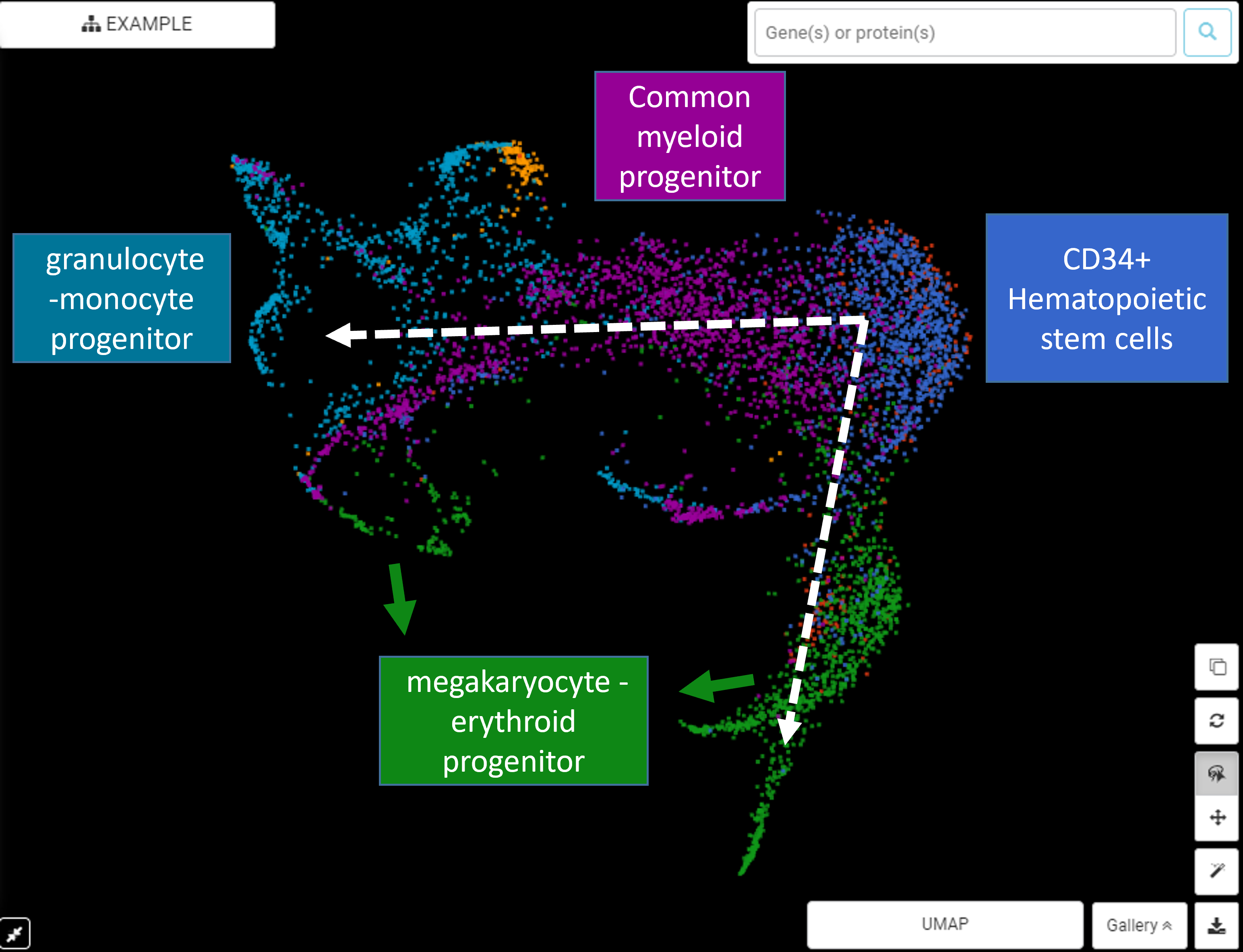
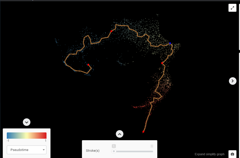
Figure 2. (upper) BBrowser’s reduced dimensional plot for Pellin et al., (2019) shows 2 possible trajectories for the differentiation of HSC to CMP, GMP, and MEP. (lower) BBrowser’s single-cell RNA-Seq trajectory analysis and pseudotime estimation for the transition from HSC to CMP, GMP, and MEP

Example #2 (Figure 3): Figure 3 (upper) is the UMAP plot for Ma et al., (2019)’s data about liver cancer cells. It’s clear that there’s no biological foundation for a trajectory connecting these cell types. The UMAP plot also depicts cell types as distinct clusters with no intermediate states. However, we can still force a trajectory analysis upon these cells to yield a meaningless trajectory (Figure 3, lower) e.g a trajectory was drawn from epithelial cells -> T cells -> myeloid cells -> B cells, depicting no sensible biological process.

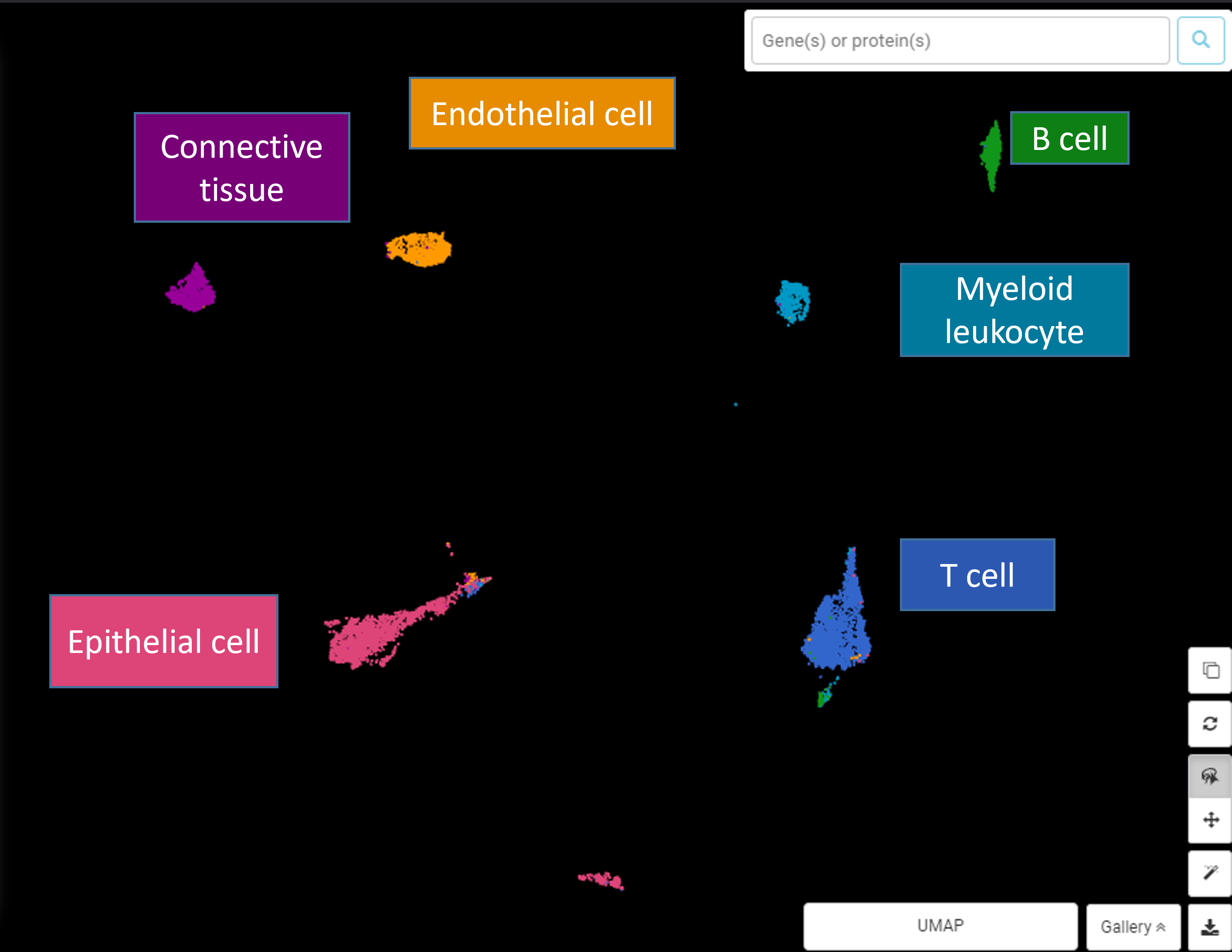
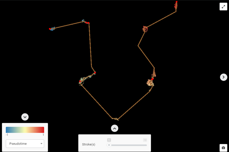
Figure 3: (upper) An example for when single-cell RNA-seq trajectory analysis is unsuitable (data from Ma et al., 2019, UMAP plot made by BBrowser). (lower) The trajectory analysis is meaningless

Example #2 also highlights a common pitfall with single-cell trajectory analysis: any dataset can be mapped into a trajectory analysis without biological meaning! 

A summarized guideline for picking a suitable Single-cell RNA-Seq Trajectory Analysis tool 

Saelens et al.(2019) performed an extensive benchmarking study to compare 45 single-cell RNA-Seq trajectory analysis tools and concluded a guideline for picking a suitable one. In this study, the authors evaluated methods in 4 criteria: (1) accuracy, using 110 real and 229 synthetic datasets with known trajectories as references, (2) scalability i.e. the number of cells and features that a method can handle, (3) stability across subsamples, and (4) user-friendliness. 

Here are the most important notes: 

• There is no one-size-fits-all tool for every dataset. 
• The topology of the trajectory largely influences a tool’s performance. There are 7 possible topologies (Figure 6). Trajectory tools are therefore classified based on what topologies they can infer (Figure 7), along with an overall evaluation result.  
• The choice of trajectory analysis tool is primarily dependent on the expected topology. Figure 8 quickly captures how users can pick a suitable trajectory analysis tool from the assumed topology. 
• However, there’s good complementarity among methods. When the topology of the trajectory is unknown (lack of prior knowledge), testing different methods is recommended. 
• Even when the trajectory’s topology is known, researchers are still recommended to test different methods. Either the expected trajectory is confirmed, or more complex trajectories may get discovered. 

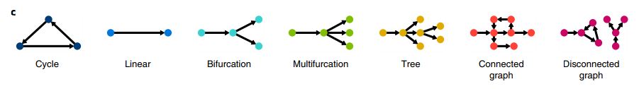
Figure 6. The 7 types of possible topology for a trajectory (Saelens et al.,2019).

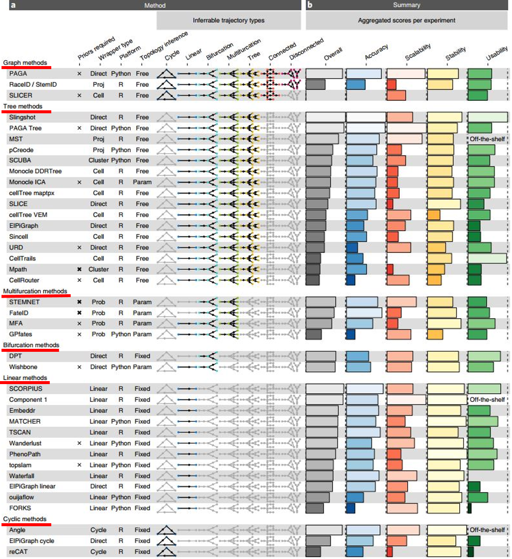
Figure 7. Single-cell RNA-Seq Trajectory analysis tools are grouped based on their most complex inferrable topology (vertical: cyclic methods, linear methods, bifurcation methods, multifurcation methods, tree methods, and graph methods). The (b) panel summarizes the overall evaluation and the particular scored on 4 criteria (Saelens et al.,2019).

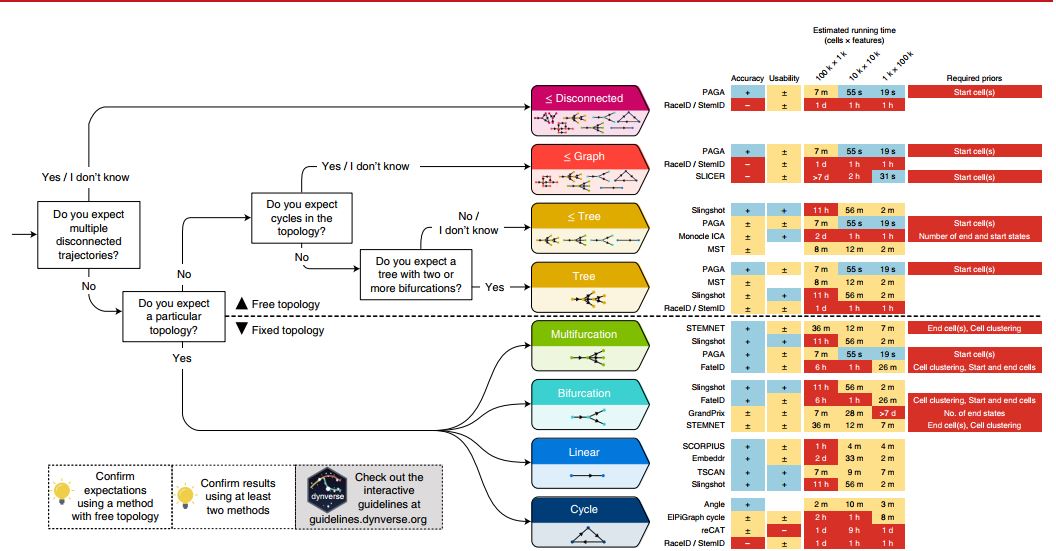
Figure 8. A quick practical guideline for picking a suitable Trajectory Analysis method (Saelens et al.,2019). Users can also access an interactive version of the guideline for easier decision-making. Since a method’s performance is largely influenced by the topology of the trajectory, users should use this as the clues. Methods are ordered from top to bottom based on their performance on a particular topology. On the right side of each method shows the 4 criteria: the accuracy (+: scaled performance ≥ 0.9, ±: >0.6), usability scores (+:≥0.9, ± ≥0.6), estimated running times and required prior information. k, thousands; m, millions. On the left bottom, users are reminded to confirm the result by trying different methods 

Reference: 

• Herring, C. A., Chen, B., McKinley, E. T., & Lau, K. S. (2018). Single-cell computational strategies for lineage reconstruction in tissue systems. Cellular and molecular gastroenterology and hepatology, 5(4), 539-548.
• Pellin, D., Loperfido, M., Baricordi, C., Wolock, S. L., Montepeloso, A., Weinberg, O. K., … & Biasco, L. (2019). A comprehensive single cell transcriptional landscape of human hematopoietic progenitors. Nature communications, 10(1), 1-15.
• Xavier-Ferrucio, J., & Krause, D. S. (2018). Concise review: bipotent megakaryocytic-erythroid progenitors: concepts and controversies. Stem Cells, 36(8), 1138-1145.
• Ma, L., Hernandez, M. O., Zhao, Y., Mehta, M., Tran, B., Kelly, M., … & Wang, X. W. (2019). Tumor cell biodiversity drives microenvironmental reprogramming in liver cancer. Cancer cell, 36(4), 418-430.
• Saelens, W., Cannoodt, R., Todorov, H., & Saeys, Y. (2019). A comparison of single-cell trajectory inference methods. Nature biotechnology, 37(5), 547-554.