In the previous post, we talked about how to visualize single-cell RNA Sequencing (scRNA-seq) data to gain meaningful insights. But there are many steps from raw sequencing data to such beautiful visualization (and further analysis) that decide whether or not researchers can make sense of their data. They include preprocessing of raw sequencing data, quality control, correction, and normalization (Luecken et al., 2019). Of all these steps, normalization is vital to several downstream analyses, especially in finding differentially expressed genes – the must-have information in every scRNA-seq study.
There are many excellent methods, however, their underlying assumptions and the type of scRNA-seq data that you’re working with will greatly decide the accuracy (Evans et al., 2018). That’s why we’re here to help! In this article, we’ll guide you through the maze of scRNA-Seq normalization methods. But first, let’s start with the basics.
1. The basics of scRNA-Seq Normalization
1.1. What is scRNA-Seq Normalization?
During the sequencing process, many technical factors can introduce bias into the raw read counts. These factors include gene length, GC-content, sequencing depth, dropouts, etc. The consequence is that the raw counts do not accurately reflect the level of biological gene expression. Technical differences between sequencing platforms could therefore introduce noise that obscures underlying biological differences between samples, making any interpretation from unnormalized data unreliable.
The goal of scRNA-seq normalization is to eliminate such technical noise or bias so that observed variance in gene expression variance primarily reflects true biological variance
1.2. Why is scRNA-Seq Normalization Needed?
The need for normalization is not unique to scRNA-seq data analysis. Long before that, many normalization methods were developed for gene expression studies using RT-PCR (reverse transcription polymerase chain reaction), RNA microarray, bulk RNA sequencing, etc. Consider the example below to understand more about the necessity of scRNA-Seq normalization.
Here is the sub clustering of the macrophage population from a study in human and mouse lung cancer (Zilionis et al., 2019), coloring by the expression level of S100A9, whose product is a critical modulator of inflammatory response (Wang et al., 2018). Figure 1 is the result from raw value, done by BBrowser. It’s easier to see that S100A9 raw expression value is highly correlated to total counts: the center of both plots have low value in counts and expression, while the peripheral area has higher counts and expression. The only conclusion we could make is that the number of S100A9 transcripts goes up when the total transcripts captured in a cell goes up. This is obviously not noteworthy. Thus, for any population whose total counts (i.e. sequencing depth) varies greatly like this, normalization is a must.
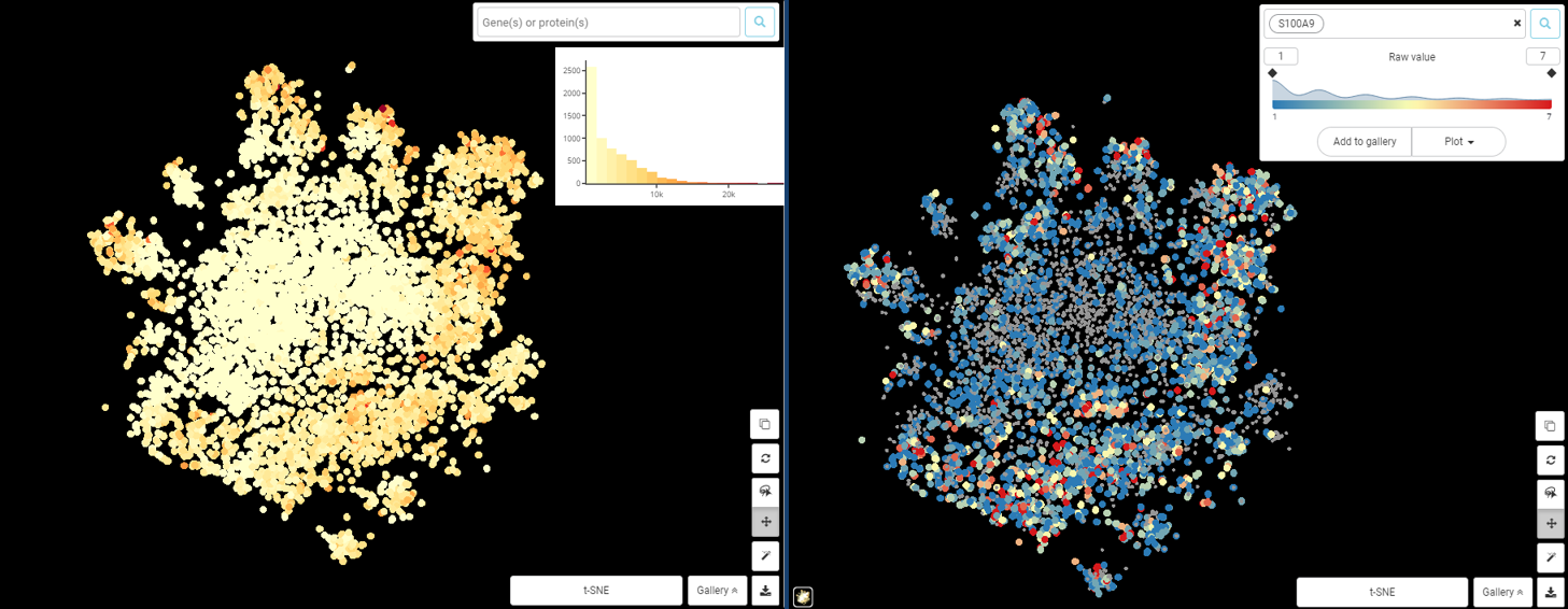
Figure 1. t-SNE plot of macrophage from Zilionis et al dataset, colored by total counts (left) and S100A9 expression based on raw value (right).
To continue with the above example, now that we already see there is great difference in total counts among this population, the logical next step would be to see if the observed difference in S100A9 is still present even after taking into account total-count disparity. Figure 2 shows how scRNA-seq normalization changed S100A9 expression pattern: there seems to be no correlation between S100A9 expression value and total counts. We can say that the variance of S100A9 expression is not dependent on technical noises like sequencing depth and should arise from (mostly) biological factors.
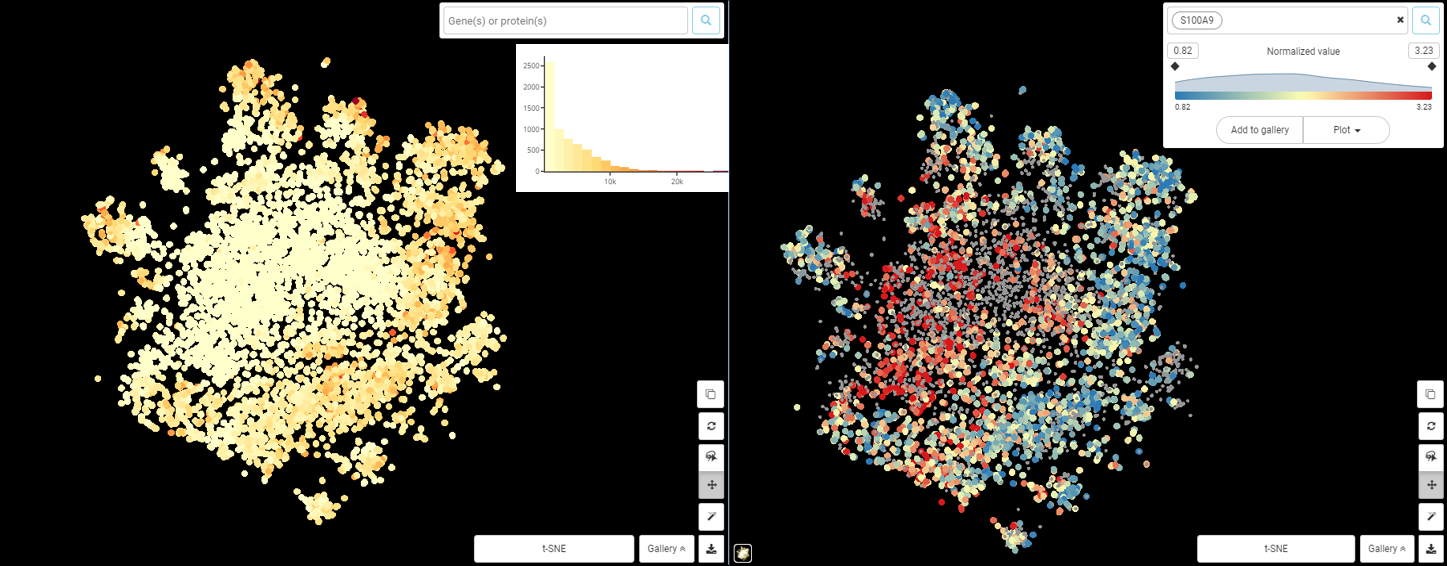
Figure 2. t-SNE plot of macrophage from Zilionis et al dataset, colored by total counts (left) and S100A9 expression based on normalized value (right).
1.3. How Does scRNA-Seq Normalization Work?
In essence, while methods vary, normalization usually happens in two steps:
- First, we apply a size factor to scale data. This step basically turns absolute counts into “concentration” – how many transcripts of gene X are there per cell (or per 10,000 or 10 millions of total counts)? This relative number is easier to deal with, comparable across cells, and is less dependent on technical variation.
- Second, normalized values are often transformed to reduce the skewness in their distribution and/or to further regress technical variation. The simplest type of transformation is log-transformation. The base for log transformation can be natural, 10, or 2, the choice of log base depends on your data value range. A more complicated type of transformation if Pearson residual, such as the one used in sctransform that we’ll discuss below.
In the next part, we’ll guide you through common scRNA-seq normalization methods. You’ll learn what are their underlying assumptions, how they normalize your data, and what you can expect in the end.
2. Common scRNA-Seq Normalization Tools and Their Principles
2.1. LogNorm
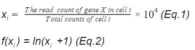
This is the default normalization method in the popular package Seurat. It’s also the default method in BBrowser’s data analysis pipeline. The principle is straight-forward: “Feature counts for each cell are divided by the total counts for that cell and multiplied by the scale.factor (default = 104 ). This is then natural-log transformed using the function log1p”.
The method can be demonstrated by two following equations. If xi is the normalized gene expression value of gene X in cell i, xi is calculated as Equation 1. The log transformation is done as Equation 2.
In other words , the gene expression measurements for each cell is normalized over the total expression i.e. the library size. The effect of varied sequencing depths between cells to cells is thus eliminated, as shown previously in Figure 1 and 2.
The default scale.factor is 104 for a simple reason: after the division, without multiplying with the scale factor, the log transformation will return difficult-to-read numbers on plots. For instance, a cell has the read count of 100 and the total count of the library is 20,000, then the normalized value without scaling is 0.0049 – not so easy to demonstrate on plots or to be comprehended. The situation is worse considering that most cells have less than 100 read counts. By applying the scale factor of 10,000, the normalized value in this case is 3.9 – seems easier for us to draw plots and have a sense of the number.
Finally, using ln(1+x) instead of natural logarithm is simply to avoid zero counts. Since zero counts are not uncommon in scRNA-seq data, without adding 1 to the normalized value, the natural log transformation will hit error most of the time.
2.2. CPM/RPM, TPM, RPKM/FPKM: old but gold
All of these terms refer to conventional bulk-RNA sequencing data normalization. An excellent and detailed explanation of these methods can be found here. In short:
- CPM (Counts per Million mapped reads) or RPM (Reads per Million mapped reads) use a scaling factor of total read counts divided for 106 (instead of the library size like LogNorm). CPM/RPM works fine when gene length has little to no impact.
- RPKM (Reads Per Kilobase Million) or FPKM (Fragments Per Kilobase Million) takes the effect of gene lengths into consideration. These methods divide the RPM by the gene length, in kilobases. The main difference is that FPKM is made for paired-end RNA-seq, in which two reads can come from a single fragment, and FPKM can avoid counting the same fragment twice.
- TPM (Transcripts Per Kilobase Million) is the same as RPKM/FPKM, but it divides the read counts by the gene length (in kilobase) first, then divides the total counts by 106 to make the scaling factor. In essence, that means to normalize gene length first, then sequencing depth.
While LogNorm and CPM are easy to use, it’s not suitable for non-UMI data because it doesn’t account for technical bias arising from different gene lengths and/or amplification efficiency.
LogNorm and above methods work well under the assumption that the amount of RNA is the same in all cells and a uniform scaling factor is applicable for all genes. However, if this is not the case, these methods may fail to detect true differential expressed genes. Genes with weak to moderate expression tend to get overcorrected, while genes with high expression get undercorrected.
2.3. SCnorm: gene group-specific scale factor
Due to the limit of global scale factors, alternatives for more accurate scale factors have been developed. An out-of-the-box solution was introduced by Bacher et al., (2017) called SCnorm.
In short, SCnorm first filters out low expression counts, then estimates the relationship between counts and sequencing depths with quantile regression. Genes with similar count-depth relationships are grouped together. Each group is given a scale factor to normalize gene expression. Problem solved!
However, users should be aware that this method ignores zero values while scRNA-Seq data is notoriously known for high drop-out rate, dampening its effect (Hafemeister and Satija, 2019).
2.4. Sctransform: normalization and variation control in one place
Sctransform is a new part of the toolkit Seurat that combines modeling, normalization, and variance stabilization in one (Hafemeister and Satija, 2019). The principle can be summarized in simple terms as followed:
- Sctransform is based on the observation that there seems to be an almost linear relationship between the UMI counts and the number of genes detected in a cell.
- The method fits a generalized linear model for UMI counts as the response variable and sequencing depth as the explanatory variable. This model describes the influence of technical noise (sequencing depth) on UMI counts.
- From the parameters computed by the above model, each UMI count is transformed into a Pearson residual, telling us how much each count is deviated from the true mean expression. The transformed UMI count is used as the normalized value.
sctransform provides an excellent tool to not only normalize data, but also stabilize variance and regress unwanted variation. However, the biggest limit of sctransform is that it’s only applicable to UMI-based scRNA-seq data due to the nature of the workflow.
In A Nutshell: Things You Should Consider When Normalizing Your Data
- What cell-specific / gene-specific effects that your data may suffer from? Consider the list below from Vallejos et al. (2017) (Table 1). Using some controls from the beginning, such as spike-ins, house-keeping genes, or opt to UMI-based platforms can help regress out some forms of technical bias. These effects will also decide which normalization method is most suited to your needs.
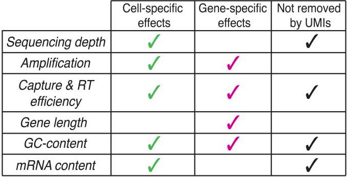
Table 1. List of effects in scRNA-Seq and the mitigation of UMI (originally Figure 1c, Vallejos et al., 2017)
- Do you assume or know that the amount of mRNA per cell is the same? If yes, methods based on a global scaling factor is good enough. If your experimental conditions may result in different mRNA per cell between conditions, you should use methods that can adjust the scaling factor flexibly, such as sctransform or SCnorm.
Closing
So far we have given the gist of scRNA-Seq normalization and introduced most popular choices, along with considerations to make the best choice for your data.
Have we answered your questions? Let us know if you need more help in the comment.
References
- Luecken, M. D., & Theis, F. J. (2019). Current best practices in single‐cell RNA‐seq analysis: a tutorial. Molecular systems biology, 15(6), e8746.
- Evans, C., Hardin, J., & Stoebel, D. M. (2018). Selecting between-sample RNA-Seq normalization methods from the perspective of their assumptions. Briefings in bioinformatics, 19(5), 776-792.
- Zilionis, R., Engblom, C., Pfirschke, C., Savova, V., Zemmour, D., Saatcioglu, H. D., … & Klein, A. M. (2019). Single-cell transcriptomics of human and mouse lung cancers reveals conserved myeloid populations across individuals and species. Immunity, 50(5), 1317-1334.
- Wang, S., Song, R., Wang, Z., Jing, Z., Wang, S., & Ma, J. (2018). S100A8/A9 in Inflammation. Frontiers in immunology, 9, 1298.
- Lytal, N., Ran, D., & An, L. (2020). Normalization methods on single-cell RNA-seq data: an empirical survey. Frontiers in genetics, 11, 41.
- Bacher, R., Chu, L. F., Leng, N., Gasch, A. P., Thomson, J. A., Stewart, R. M., … & Kendziorski, C. (2017). SCnorm: robust normalization of single-cell RNA-seq data. Nature methods, 14(6), 584-586.
- Hafemeister, C., & Satija, R. (2019). Normalization and variance stabilization of single-cell RNA-seq data using regularized negative binomial regression. Genome biology, 20(1), 1-15.
- Vallejos, C. A., Risso, D., Scialdone, A., Dudoit, S., & Marioni, J. C. (2017). Normalizing single-cell RNA sequencing data: challenges and opportunities. Nature methods, 14(6), 565-571.