Clustering is The Microscope For scRNA-Seq data
In previous posts, we have walked you through important steps in analyzing your single-cell RNA sequencing (scRNA-Seq) data, including data visualization and normalization. This time, let’s explore the next logical step in the data analysis pipeline: clustering scRNA-Seq data.
What is scRNA-Seq clustering?
It is an unsupervised machine learning step to group cells based on their similarities in gene expression profile. From clustering results, hidden patterns emerge, giving us insights into scRNA-Seq data and potential confounding factors.
Often, clustering goes hand in hand with cell type annotation. Groups of similar cells are identified and annotated to cell types/ subtypes. The outcome of clustering scRNA-Seq data is a nice partition of the huge and unordered initial dataset, which is more digestible to the human brain. Thus, clustering helps you to zoom in your scRNA-Seq data like a microscope and find interesting observations through noises.
Why must we perform scRNA-Seq clustering analysis?
Imagine that you’re now having a bunch of individual cells and their transcriptomes but have no idea about their identities. Without this information, how do you associate observations with biological meanings? Clustering comes to your rescue: by dividing cells into distinct groups (plus identifying them), you have a clue on investigating further. Which groups (aka cell type/ cell state) express unique genes? Exhibit interesting pathways? Present in a strange phenomenon? And so on.
A great example of the benefit from scRNA-Seq clustering analysis is exploring intratumoral heterogeneity: by discovering novel cell subtypes, researchers can unravel unique developmental pathways, disease progress, treatment resistance, etc. (Figure 1).
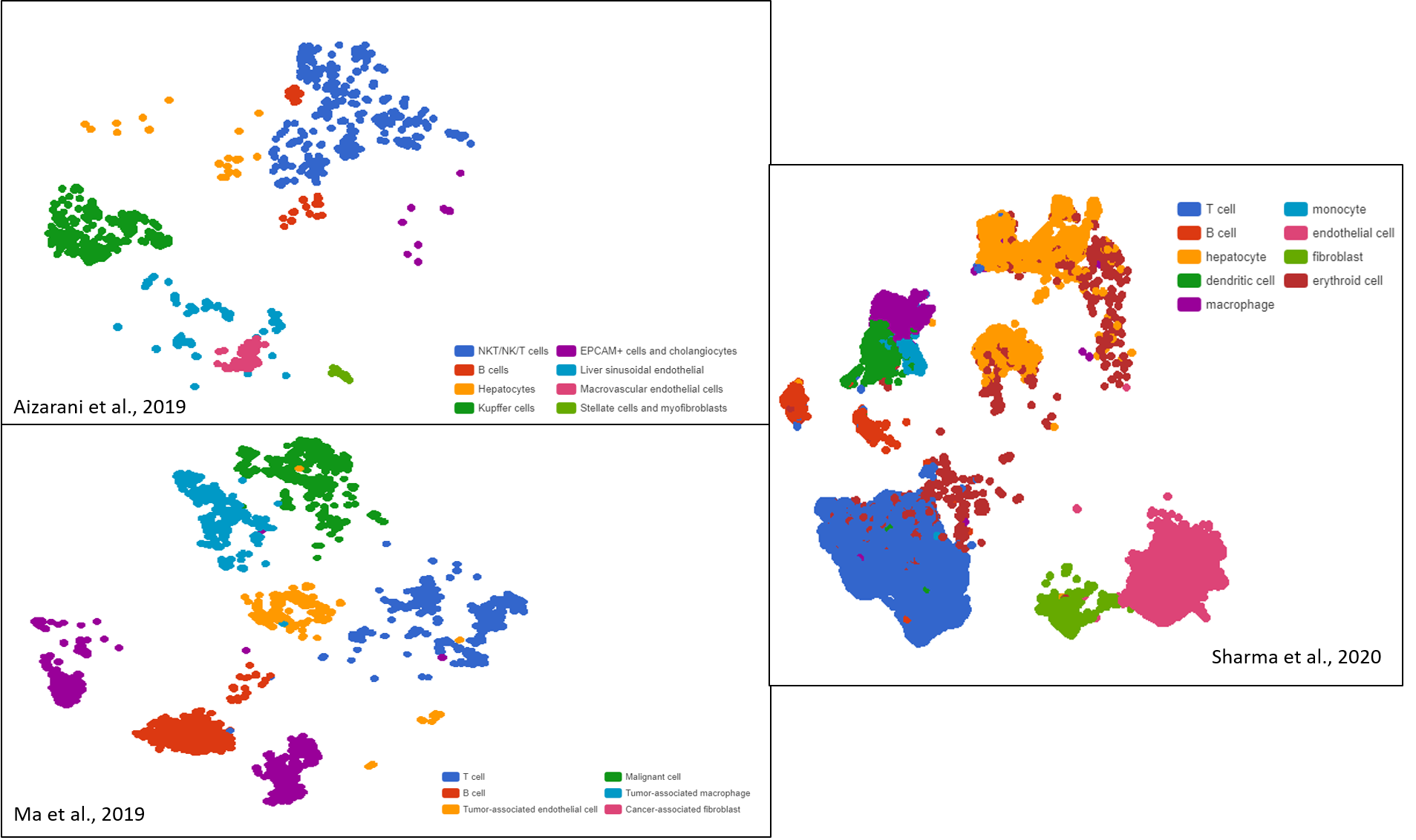
Figure 1. Liver cancer cell compositions of three different datasets exhibit high diversity after clustering, visualized as t-SNE and UMAP plots by BBrowser
In this article, let us give you some ideas on how to do scRNA-Seq clustering right.
The Common Goal of scRNA-Seq Clustering Methods
Regardless of the implementation, clustering methods aim for the same goal: to divide a dataset into groups so that within-cluster cells are as similar as possible, while between-cluster differences are maximized.
There are several scRNA-Seq clustering methods, but they can all be grouped into one of the following classes, or a combination of two or more:
- Hierarchical
- k-means
- Graph-based
- Gaussian mixture
- Mean shift
Most popular scRNA-Seq clustering tools are based on the first three classes. Each has their pros and cons, which have been examined in an excellent review from Kiselev et al., (2019). A summary of scRNA-Seq clustering tools and their characteristics is present in Table 1.
For BBrowser, the method of choice is the Louvain algorithm – a graph-based method that searches for tightly connected communities in the graph. Some other popular tools that embrace this approach include PhenoGraph, Seurat, and scanpy. Simply put, this algorithm first constructs a graph using cells as nodes. Cells with similar transcriptomes are connected by edges. The Louvain algorithm then clusters cells by trying to divide the graph so that the modularity is maximized. This method outperforms other classes when dealing with large datasets in terms of speed and accuracy (Kiselev et al., 2019).
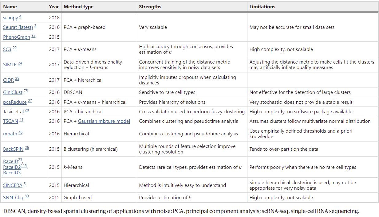
Table 1. Popular scRNA-Seq clustering tools and their classification, pros, and cons (originally Table 1, Kiselev et al., 2019)
How to Get The Informative Clusters?
Getting clusters is not the end – you have to make sense of them! The danger is here: we don’t know what the “real” clusters look like because clustering is an unsupervised machine learning process.
To make things more complicated, there can be many ways to cluster a dataset: you can divide and group cells in different ways depending on which angle you would like to look at them. Take a look at an example from Zhang et al., (2019). In this study, the dynamic landscape of immune cells in liver cancer tissue was explored and described in detail. The result from graph-based clustering yields 29 clusters, but not all of them are interesting or meaningful (Figure 2).
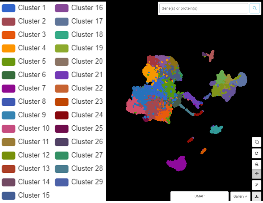
Figure 2. BBrowser graph-based clustering result for Zhang et al. (2019) dataset in immune cells from liver cancer tissue.
Upon further investigation, the authors can regroup and identify 9 clusters for major immune cell types (Figure 3). These clusters are much more informative than the initial graph-based result.
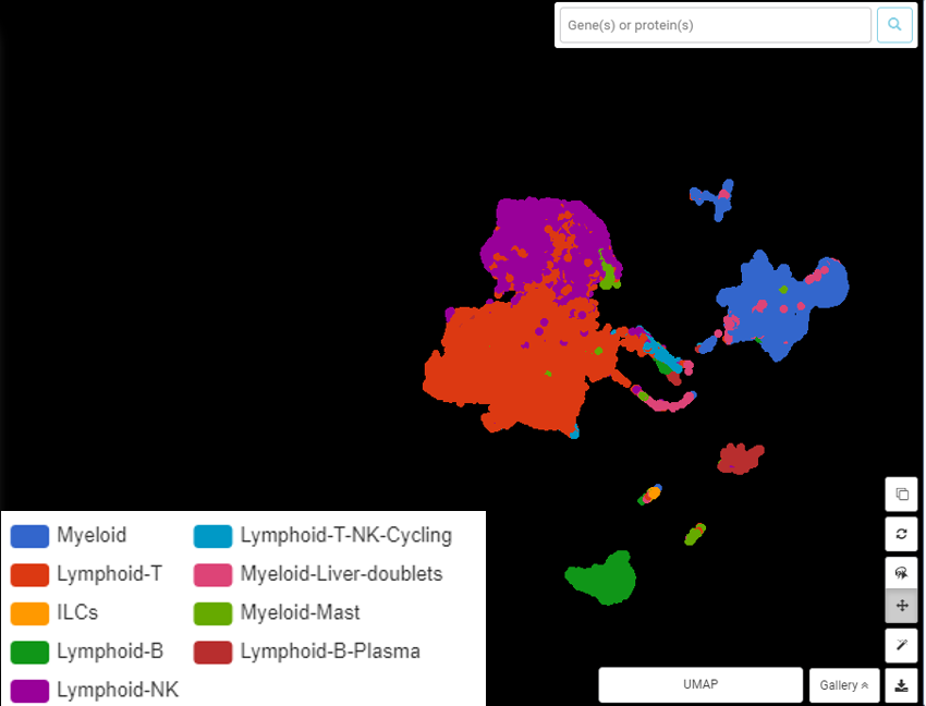
Figure 3. Regrouping and annotation by marker genes resulted in 9 clusters for 9 immune cell types. UMAP presentation done by BBrowser
But the job is not done yet. From these 9 clusters, the dataset can still be split further, revealing 40 clusters for 40 cell subtypes (Figure 4)! This information opened up a novel landscape of immune cells in hepatocellular carcinoma.
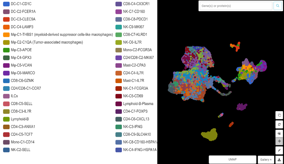
Figure 4. The diverse immune cell populations in hepatocellular carcinoma revealed by clustering. UMAP presentation done by BBrowser
So how do we get the right clusters that promise biological meanings upon further analysis? Here are some considerations.
1. Take Quality Control Seriously
Technical biases can misguide your clustering results from the beginning. What you end up getting is clusters differed by things like batch effects, low number of genes captured, high mitochondrial content, etc. not by biological phenomena. Before running clustering analysis, make sure you have preprocessed your data. When your clustering doesn’t seem to make sense, revisit and modify your quality control parameters to filter out junk information.
From BBrowser 3, our data analysis pipeline gives users flexibility in tuning your QC parameters, including interactive preview of raw data, adjustable key filters, and a range of batch effect removal options.
2. Dimensionality Reduction before Clustering
Since clustering is an unsupervised machine learning process, if performed on the original data, the result often needs to be reexamined to remove redundant features and to correct meaningless clusters. This stems from the Curse of Dimensionality: the high dimensional space makes cells so sparse that they all appear dissimilar.
That said, applying dimensionality reduction techniques not only speeds up clustering algorithm(s) by moving cells closer, but also results in more reliable clusters.
However, one needs to be careful with what dimensionality reduction methods to use before clustering. Principal Component Analysis (PCA) is often recommended because it works to retain the most variance in a dataset. In the BBrowser data analysis pipeline, clustering is done on PCA results.
Dimensionality reduction techniques like t-SNE and UMAP are also a good choice but since their primary goal is to visualize data in the clearest way possible, their partition of the dataset is not always meaningful.
3. Get The Right Number of Clusters
This is probably the hardest criterion to find. So far, there hasn’t been a consensus answer, but there are some ideas that prove to be useful.
For instance, bootstrapping is a fairly simple test. After clustering, take a random subsample and repeat clustering multiple times to see if you frequently receive the same structure. However, this trick only proves that the computational process is reproducible.
Optimizing clustering parameters is another way to come closer to the truth. For example, in the graph-based approach embraced by BBrowser, “resolution” is a critical parameter, which determines the number of clusters (higher resolution value will return more clusters). Within the Seurat package, the FindClusters() function allows users to test and play with a range of resolutions. The results are visualized by t-SNE or UMAP, so that users can find the optimal resolution by judging how well and clear a dataset is partitioned. In addition, there are also tools developed just to optimize this parameter, such as clustree.
In Summary
Clustering is the key step in unveiling the biological insights of your scRNA-Seq data. At the same time, this step is quite tricky and there is no fixed way to do it correctly. In this article, we have discussed some tricks to help you figure out the optimal clustering results.
Nevertheless, the biological context is your ultimate guide. You should:
- Have some expectations / predictions of what cell types should be present before clustering. Use this knowledge as your guidance when examining the clustering result.
- Use the differentially expressed (DE) genes in your clusters to identify the enriched biological process(es) for each cluster. From here, you have a cue to either split the dataset further or regroup clusters.
- One rising strategy is to cross-check your novel clusters with annotated data. Comprehensive cell atlases and cell ontology databases are some useful resources to validate your clustering results.
Reference:
Kiselev, V. Y., Andrews, T. S., & Hemberg, M. (2019). Challenges in unsupervised clustering of single-cell RNA-seq data. Nature Reviews Genetics, 20(5), 273-282.
Zhang, Q., He, Y., Luo, N., Patel, S. J., Han, Y., Gao, R., … & Zhang, Z. (2019). Landscape and dynamics of single immune cells in hepatocellular carcinoma. Cell, 179(4), 829-845.