Differential expression analysis is a common step in a Single-cell RNA-Seq data analysis workflow. In our previous post, we have given an overview of differential expression analysis tools in single-cell RNA-Seq. This time, we’d like to discuss a frequently used tool – DESeq2 (Love, Huber, & Anders, 2014).
According to Squair et al., (2021), in 500 latest scRNA-seq studies, only 11 methods made up to over 80% of DE analysis. DESeq2 ranks second.
What makes DESeq2 a widely popular tool in single-cell analysis? In this article, we’ll break down the basics of DESeq2 and highlight 2 advantages of DESeq2 in differential gene expression for single-cell RNA-seq.
DESeq2’s oversimplified procedure
Here’s an oversimplified description of what DESeq2 does stepwise and what each step means.
First: calculate the mean and estimate the dispersion of gene expression for each and every gene. The highlight of this step is the estimation of dispersion, a statistic reflecting the relationship between mean and variance. Due to the nature of single-cell RNA seq data, the ratio of mean and variance shifts when the expression level of a gene changes rather than remains constant, thus it is important to accurately estimate the relationship between these two statistics via dispersion for subsequent model fitting step.
Second: with the dispersion estimated, the count value of each gene is fitted to a Negative Binomial Generalized Linear Model (Formula 1). While the exact details for the fitting could be found in linked articles at the end of the blog, the end result is coefficients that represent expression change between conditions/samples (i.e log fold changes) (Formula 2, 3).
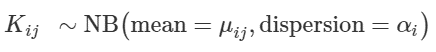
Formula 1: The read count Kij (for gene i in sample j) is fitted to a Negative Binomial GLM with two parameters mean expression value and dispersion (which we have calculated and estimated in step 1)
![]()
Formula 2: An easier interpretation of the Negative Binomial GLM in Formula 1 with y is the gene expression (obtained from the mean and dispersion), xi is the design factor i (e.g control = 0, case = 1), ẞi is the coefficient for design factor i (explained in detail here). This is also called the Design Formula, which users must specify before running DESeq2.
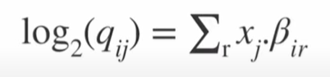
Formula 3: After fitting, the coefficient ẞi provides information about the log fold change. In particular, the log fold change in the expression of gene i in sample j is calculated from the sum of fold changes related to all design factors taken into account
Finally: run a statistical test to examine if the changes are statistically significant. Here we have two options: the Wald test or the Likelihood Ratio test
The Wald test is a pairwise comparison where the null hypothesis is that the log fold change (the gene model coefficient) is zero, indicating no significant differential expression between two groups.
The Likelihood Ratio Test, on the other hand, aims to compare two models to see which one better explains the observed data. These two models both contain confounding variables that need to be accounted for, yet the more complex one (i.e., the full model) also contains the variable of interest. The basic idea of this test is to see if, by the addition of another variable (the variable of interest), the full model can do a better job fitting to the data at hand. If not, then we are better off with the simpler model (Occam’s razor). For single cell RNA seq data, it is recommended this second test is used over the Wald test [ref].
Two Reasons Why DESeq2 Is A Widely Popular Choice in Differential Expression Analysis for Single-cell RNA-Seq
#1 Good estimation of variance through the gene-wise dispersion parameter of Negative Binomial distribution
Negative Binomial Distribution is a good choice for count-based, multimodal, overdispersed data (i.e. when the variance is much greater than the mean). This is suitable for RNA-seq data in general, where variance comes from several sources, both technical and biological.
But what’s important here are the two parameters of NB distribution: the mean and the dispersion. The dispersion is a function of the mean and variance, thus it helps estimate the variance for a given mean value. Remember that getting an accurate estimation of expression variance is critical in finding DE genes.
Here, we would like to emphasize the strength of DESeq2 and similar tools, notably edgeR (Robinson, McCarthy, & Smyth, 2010), in dispersion estimation, which makes them popular choices when it comes to count modeling of single-cell RNA-seq data.
First, a dispersion value is estimated for each gene, using data from that gene only. Yet often this estimate is not reliable enough to be fed directly into the subsequent fitting step, so DESeq2 assumes that genes with similar expression levels have similar dispersion i.e. using information from all genes.
With this assumption, it is justifiable to fit a curve to all the gene-wise estimates from the previous step, and use that curve to improve our dispersion estimates (intuitively speaking, using information from genes of similar expression profiles to better estimate the current gene’s statistics). The way DESeq2 does that is by shrinking each of them towards the mean values, as illustrated by the direction of the arrow in Figure 1.
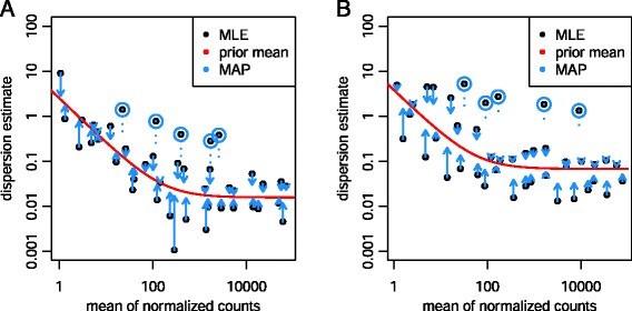
Figure 1: Shrinkage estimation of dispersion. Originally figure 1, Love, Huber, & Anders, (2014)
It’s worth emphasizing that the curve above allows for more accurate identification of differentially expressed genes when sample sizes are small, and the strength of the shrinkage for each gene depends on how close gene dispersions are from the curve, and sample size (more samples = less shrinkage). The shrinkage is also important for checking the fitness of our data. If the fitting is not so successful, users need to re-examine data to find out if there’s any variance besides biological factors that cause such great dispersion.
#2 A generalized linear model (GLM) that accounts for possible confounding effects
A common problem in DE analysis is that confounding effects (such as gender, age, organ, etc.) can mask DE genes caused by the variable of interest (such as cell types, disease, treatment, etc.)
DESeq2 and similar methods solve this by fitting each gene’s expression in a generalized linear model (Negative Binomial regression) that accounts for these possible confounding effects. The highlight is users can specify which variables are confounding factors and which one is the variation of interest. Moreover, users can also investigate the interaction between variances. For a more in-depth explanation of how to define the formula to be fitted by DESeq2 and how to interpret the resulting coefficients after the fitting is done, motivated readers are recommended to head to other tutorials here and here.
We hope this article has given you everything you need to know about the basics of DESeq2. The method is available in BBrowser’s Differential Expression Analysis toolkit, along with our in-house algorithm Venice and other equally popular algorithms (Wilcox, Likelihood-ratio test, T-test, Logistic regression). Our simple UI helps users run diferential expression on single-cell data in a few clicks (Figure 2) (refer to BBrowser user guide on differential expression analysis)
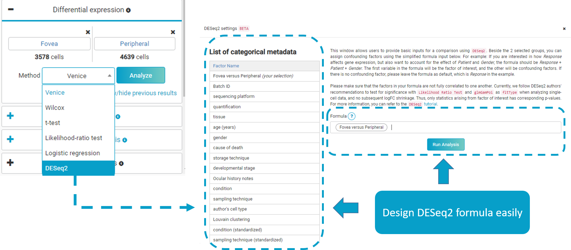
Figure 2. Run DESeq2 and other popular differential expression analysis at ease in a few steps with BBrowser. Simply pick two groups, choose a method, and adjust parameters. For DESeq2, users can choose which variable/design factor to include in the design formula (Formula 2), keeping in mind that the first variable is the variable of interest, while the rest are confounding factors
Below is an example on BBrowser performing DESeq2 differential expression analysis on single-cell RNA-seq data between foveal and peripheral human retina cells, based on the study of Voigt et al. (2019), to distinguish the transcriptomic features between the two groups (Figure 3).
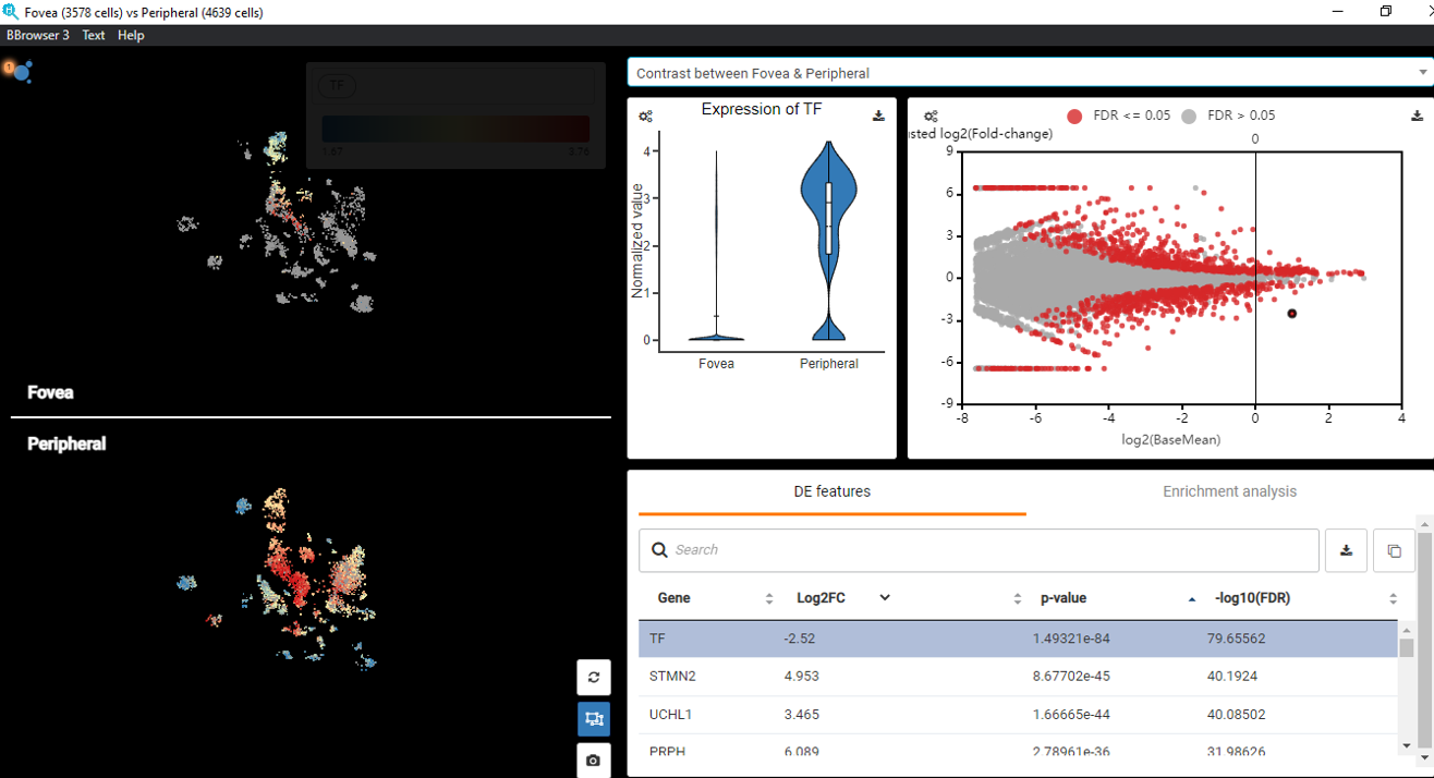
Figure 3. BBrowser performed DESeq2 on the dataset of Voigt et al., (2019) to distinguish the transcriptomic profiles of foveal versus peripheral human retinal cells
Reference:
- Love, M. I., Huber, W., & Anders, S. (2014). Moderated estimation of fold change and dispersion for RNA-seq data with DESeq2. Genome biology, 15(12), 1-21.
- Squair, J. W., Gautier, M., Kathe, C., Anderson, M. A., James, N. D., Hutson, T. H., … & Courtine, G. (2021). Confronting false discoveries in single-cell differential expression. Nature communications, 12(1), 1-15.
- Robinson, M. D., McCarthy, D. J., & Smyth, G. K. (2010). edgeR: a Bioconductor package for differential expression analysis of digital gene expression data. Bioinformatics, 26(1), 139-140.